Chapter 9 Generative Models

So far, we have mainly looked as Discriminative Models.

The models try to estimate the likelihood \(P(Y | X)\).

For instance, logistic regression would be a discriminative classifier.

These where all supervised learning models (the training data \({\bf X}\) is associated with given labels \({\bf y}\)).

Example 9.1 Given a dataset of labelled images, detect whether the picture is of a face or not.

Generative Models try to model the probability distributions of the data itself, ie. \(P(X)\) or \(P(X | Y)\).

The objective is to learn how to synthesise new data, that is similar to the training data.

As we don’t have ground truth data about what that data should be, it is a form of unsupervised learning (we’re just trying to learn from the data itself).

Example 9.2 Given a dataset of faces, and you would like to generate new realistic looking faces: \[ X \sim P(X | Y=\mathtt{'cat'}) \]

Popular generative models that use deep learning include:

• Generative Adversarial Networks
• Autoencoders
• Auto-Regressive Models (eg. GTP-3,4)
• Diffusion Models (eg. image generation apps like Midjourney, DallE, etc. )

In this module, we will not cover the case of diffusion models.

9.1 Generative Adversarial Networks (GAN)

Generative Adversarial Networks (or GANs) have been the most predominant method of generative models in the past years. It is only recently that diffusion models have overtaken as the method of choice.

Consider the two following problems:

A. You are asked to design an application that can generate photo portraits of people that don’t exist. Your idea is to start from a noisy image and use a sequence of conv layers to transform the noise into actual photos of (fake) people. What kind of loss function would be suitable? How can we know if an image is a realistic photo?

B. A news agency has been overwhelmed by fake photos. You are asked to design a forensic tool that can detect whether a picture is real or fake. But for training you only can put your hands on a few pictures that you know for sure were photoshoped. How can you get enough training data?

Both problems are obviously related and are at the core of Generative Adversarial Networks or GAN.

Ian Goodfellow et al. ``Generative Adversarial Network’’ (2014). https://arxiv.org/abs/1406.2661

GAN’s architecture (see Fig.9.1) is made of two NN: a Generator Network, that is responsible for generating fake data, and a Discriminator Network that is responsible for detecting whether data is fake or real.

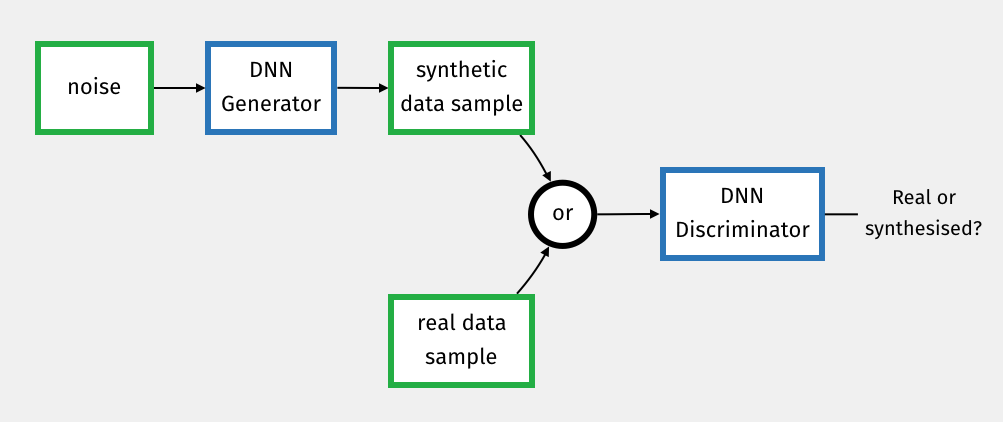
Figure 9.1: GAN Architecture

Typically the generator network takes an input noise and transforms that noise into a sample of a target distribution. This is our photo portrait generator: it transforms a random seed into a photo portrait of a random person.

The loss function for that generator is the discriminator network that in our case can classify between fake and real photos.

It is thus an arms race where each network is trying to outdo the other.

Both problems taken independently are hard because the generator is missing a loss function and the discriminator is missing data but by addressing both problem at the same time in a single architecture, we can solve for both problems.

Training GAN networks is particularly slow and difficult but the benefits are spectacular. This is a very hot topic of research.

Figure 9.2: Example of GAN generating pictures of fake celebrities (see 2018 ICLR NVidia paper here [https://goo.gl/AgxRhp]

9.2 AutoEncoders

9.2.1 Definition

So far, we have looked at supervised learning applications, for which the training data \({\bf x}\) is associated with ground truth labels \({\bf y}\). For most applications, labelling the data is the hard part of the problem.

Autoencoders are a form of unsupervised learning, whereby a trivial labelling is proposed by setting out the output labels \({\bf y}\) to be simply the input \({\bf x}\). Thus autoencoders simply try to reconstruct the input as faithfully as possible.

Autoencoders seem to solve a trivial task and the identity function could do the same. However, in autoencoders, we also enforce a dimension reduction in some of the layers, hence we try to compress the data through a bottleneck.

Fig. 9.3 shows the example of an autoencoder. The input data \((x_1,x_2,x_3,x_4)\) is mapped into the compressed hidden layer \((z_1,z_2)\) and then re-constructed into \((\hat{x}_1, \hat{x}_2, \hat{x}_3, \hat {x}_4)\). The idea is to find a lower dimensional representation of the data, where we can explain the whole dataset \({\bf x}\) with only two latent variables \((z_1,z_2)\).

Figure 9.3: Example of an Auto-Encoder.

The autoencoder architecture applies to any kind of neural net, as long as there is a bottleneck layer and that the output tries to reconstruct the input. The general principle is illustrated in Fig. 9.4.

Figure 9.4: General architecture of an Auto-Encoder.

Typically, for continuous input data, you could use a \(L_2\) loss as follows:

\[ \text{Loss}\ \boldsymbol{\hat{\textbf{x}}} = \frac{1}{2} \|\boldsymbol{\hat{\textbf{x}}} - \textbf{x} \|^2 \]

Alternatively you can use cross-entropy if \({\bf x}\) is categorical.

9.2.2 Examples

The following examples consider the MNIST handwritten digit database and are taken from the following link:

https://blog.keras.io/building-autoencoders-in-keras.html

Here is an example of autoencoder using FC layers:

encoding_dim = 32  
input_img = Input(shape=(784,))
encoded = Dense(encoding_dim, activation='relu')(input_img)
decoded = Dense(784, activation='sigmoid')(encoded)
autoencoder = Model(input_img, decoded)

Here is an example of a convolutional autoencoder:

input_img = Input(shape=(28, 28, 1))

x = Conv2D(32, (3, 3), activation='relu', padding='same')(input_img)
x = MaxPooling2D((2, 2), padding='same')(x)
x = Conv2D(32, (3, 3), activation='relu', padding='same')(x)
encoded = MaxPooling2D((2, 2), padding='same')(x)

# at this point the representation is (7, 7, 32)

x = Conv2D(32, (3, 3), activation='relu', padding='same')(encoded)
x = UpSampling2D((2, 2))(x)
x = Conv2D(32, (3, 3), activation='relu', padding='same')(x)
x = UpSampling2D((2, 2))(x)
decoded = Conv2D(1, (3, 3), activation='sigmoid', padding='same')(x)

autoencoder = Model(input_img, decoded)
autoencoder.compile(optimizer='adadelta', loss='binary_crossentropy')

Note that we use UpSampling2D to upsample the tensor in the decoder part. This upsampling stage is sometimes called up-convolution, deconvolution or transposed convolution. This step upsamples the tensor by inserting zeros in-between the input samples. This is usually followed by a convolution layer. More on this is discussed in the link below.

Just note that the word deconvolution is very unfortunate as the term deconvolution is already used in signal processing and refers to trying to estimate the input signal/tensor from the output of a convolution (eg. trying to recover the original image from an blurred image).

Below are the results of our convolutional autoencoder for the MNIST dataset. The input is on top and the reconstructions results on bottom.

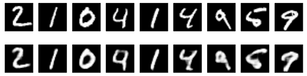
Figure 9.5: reconstruction results on MNIST.

The reconstructed results look very similar, as planned. The interest of a compressed representation is illustrated below, where the input is noisy but the decoder network reconstructs clean images.

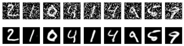
Figure 9.6: reconstruction results on noisy inputs.

9.2.3 Dimension Compression

We need however to be mindful that dimensional reduction does not necessarily imply information compression. In Fig. 9.7 is shown an example of what we are looking to do. The mapping from \({\bf x}\) into \({\bf z}\) comes with a loss of information. In this case, any variation perpendicular to the dashed line is discarded as being noise. The reconstruction \(\boldsymbol{\hat{\textbf{x}}}\) is close but slightly different from \({\bf x}\). The idea here is actually a classic concept in unsupervised learning and is actually very similar to something like Principal Component Analysis.

Figure 9.7: Example of a dimension reduction, with information compression.

However, as illustrated in Fig. 9.8, there is no guarantee that the dimensional compression leads to something meaningful. We have here a one-to-one correspondence function that can map any point in the 2D space into the 1D space and vice-versa but the resulting latent variables \(z_1, z_2\) are of probably not of much interest because the latent space is extremely entangled.

Figure 9.8: Example of a dimension reduction, without information compression.

In practice, convolution networks are fairly smooth and do not create such extreme mappings. Still, we have little control over the latent space itself, which could end up being skewed and hard to make sense of.

Let’s see that on an example for MNIST with a 2D latent space with the following network:

inputs = Input(shape=(784,))
x = Dense(512, activation='relu')(inputs)
z = Dense(2, name='latent_variables')(x)
x = Dense(512, activation='relu')(z)
outputs = Dense(784, activation='sigmoid')(x)

The bottleneck layer only contains 2 units. Thus the input \(28 \times 28\) image is mapped into two latent variables \(z_1, z_2\). Fig. 9.9 shows the 2D scatter plot of the latent variable \((z_1,z_2)\), coloured by class id. Each point \((z_1,z_2)\) in the plot represents an image from the training set. This particular mapping forms a complex partition of the space. Classes clusters are skewed, or broken into different parts, and leaving gaps where values of \((z_1,z_2)\) do not correspond to any digit.

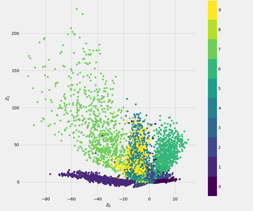
Figure 9.9: Scatter plot of the MNIST training set in the Latent Space (Encoder)

Fig. 9.10 shows the decoded images for each value of \((z_1,z_2)\). For values of \((z_1,z_2)\) outside of the main clusters, the reconstructed images become blurred or deformed.

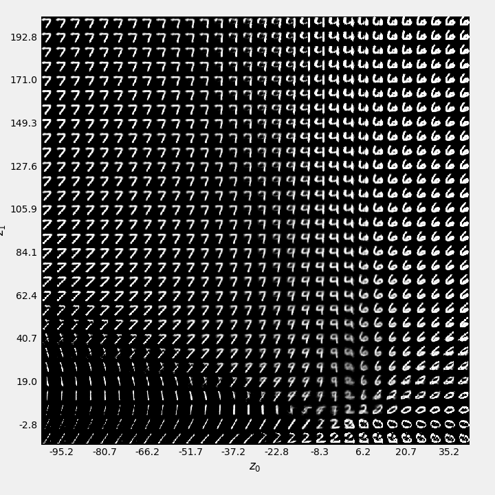
Figure 9.10: Reconstructions of the latent variables (Decoder).

The issue with AEs is that we ask the NN to somehow map 784 dimensions into 2, without enforcing anything about what the distribution of the latent variables should look like. Since the loss is only focused on the reconstruction fidelity, the latent space could end up being messy. Instead, what we are really looking for is an untangled latent space, where each latent variable has its own semantic meaning: eg. for a portrait images, \(z_1\) could control the head size, \(z_2\) the hair colour, \(z_3\) the smile, etc. Perfect aligning with the semantic labels is however probably unattainable, as semantic labels are not accessible at training time. We could, however, at least to constraint the distribution of the latent variables to be a bit more reasonable. For instance, by making sure that the \({\bf z}=0\) is the mean value of the distribution, or by making sure that its standard deviation is set to 1. This is exactely what variational auto encoders are trying to do.

9.2.4 Variational Auto Encoders (VAE)

In Variational Auto Encoders (VAEs), we impose a prior on the distribution \(p({\bf z})\) of the latent vectors \({\bf z}=[{ z}_1, \cdots, { z}_n ]^\top\). The prior is that \(p({\bf z})\) should be the normal distribution: \[ p({\bf z}) = \mathcal{N}(0, Id) \] which means that the distribution of \({\bf z}\) will be smooth and compact, without any gap.

Since we are looking to constrain the distribution \(p({\bf z})\) and not just the actual values of \({\bf z}\), we now need to manipulate distributions rather than data points. As manipulating distributions is a bit tricky and yield intractable equations, we will make some approximations along the way and resort to a Variational Bayesian framework. In particular, we are going to assume that the uncertainty \(p({\bf z} | {\bf x})\) follows a Multivariate Gaussian:

\[ p({\bf z} | {\bf x}) = \mathcal{N}(\mu_{{\bf z} | {\bf x}}, \Sigma_{{\bf z} | {\bf x}}) \]

Recall that \(p({\bf z} | {\bf x})\) models the range of values \({\bf z}\) that could have produced \({\bf x}\). What is expressed by \(p({\bf z} | {\bf x})\) is thus all the variations that are due by unrelated processes, such as signal noise and other distortions.

Figure 9.11: VAE architecture.

The optimisation of the VAE model leads to the approach described in Fig. 9.11. The exact derivations that lead to this solution go beyond the scope of this lecture material and will not be covered here. It is nevertheless interesting to look at some of the practical components of this architecture:

1. The encoder network predicts the distribution \(p({\bf z}|{\bf x})\) by directly predicting its mean and variance \(\mu_{{\bf z} | {\bf x}}\) and \(\Sigma_{{\bf z} | {\bf x}}\). As we want the distribution of \(p({\bf z})\) to be normal (ie. \(p({\bf z}) = \mathcal{N}(0, Id)\)), we define a loss function (\(\text{Loss}\ {\bf z}\)), based on the Kullback-Leibler divergence, \(D_{KL}\), to measure the difference between the predicted distribution and the desired \(\mathcal{N}(0, Id)\):

\[ \text{Loss}\ {\bf z} = D_{KL}( \mathcal{N}(\mu_{z | x},\Sigma_{z | x}), \mathcal{N}(0,Id) ) = \frac{1}{2} \sum_{k} \Sigma_{k,k} + \mu_k^2 -1 -\log(\Sigma_{k,k}) \]

2. We then sample \(z \sim p({\bf z}| {\bf x})\). Sampling is a bit tricky because this is apriori not a differentiable step. The trick is here to pre-define a random variable \(\epsilon \sim \mathcal{N}(0, Id)\) and then simply proceed to generate the sample \({\bf z}\) as follows: \[ {\bf z} = \mu_{{\bf z }|{\bf x}} + \Sigma_{{\bf z }|{\bf x}}^{\frac{1}{2}} \epsilon \] Since \(\epsilon\sim \mathcal{N}(0, Id)\), we are guaranteed that \(z \sim p({\bf z}| {\bf x})=\mathcal{N}(\mu_{{\bf z} | {\bf x}},\Sigma_{{\bf z} | {\bf x}})\).

3. The decoder then reconstructs \(\boldsymbol{\hat{\textbf{x}}}\). \[ \text{Loss}\ \boldsymbol{\hat{\textbf{x}}} = \frac{1}{2} \|\boldsymbol{\hat{\textbf{x}}} - \textbf{x} \|^2 \]

You can think of the sampling step as a way of working on distributions when in fact we are only defining the decoder network as an operation on data.

So it is all a bit complicated, but if you look at Fig. 9.12, the resulting 2D scatter plot of the latent variable \((z_1,z_2)\) is indeed much closer to a normal distribution and the class clusters are less skewed than compared to AE.

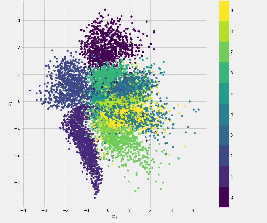
Figure 9.12: 2D scatter plot of the latent variable \((z_1,z_2)\), coloured by class id for the Variational Auto Encoder model.

The decoded images associated with each value of \((z_1,z_2)\) are shown in Fig. @(fig:AE-vae-digits-over-latent). We can see see that ill-formed reconstructions now only arise for extreme values of \((z_1,z_2)\).

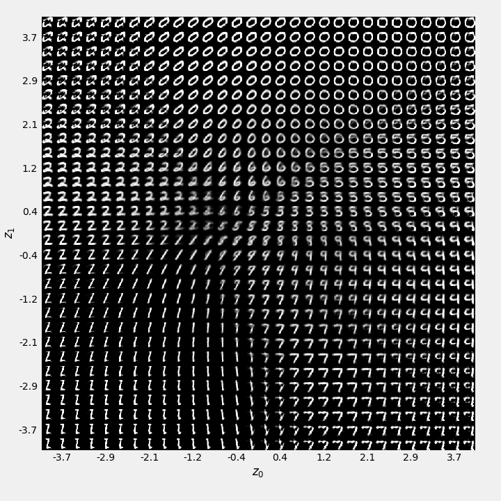
Figure 9.13: 2D scatter plot of the latent variable \((z_1,z_2)\), coloured by class id for the Variational Auto Encoder model.

9.2.5 Multi-Tasks Design

The Encoder is the key part of the autoencoder architecture. There is however only so much that can be achieved with an unsupervised method. Looking at the success of pretrained networks such as ResNet or VGG, supervised learning is arguably a much more effective way of training encoders.

An idea, that has gained popularity, is to combine multiple approaches in a Multi-Task training strategy. The approach, illustrated in Fig. 9.14, is that the same encoder can be shared across a multitude of classification tasks that are related to the application at hand. The training strategy then simply consists of alternating between the various training tasks, for a few mini-batch updates per task.

Figure 9.14: Example of a more comprehensive multi-tasks auto-encoder, including a GAN.

For instance, if your application is to generate images of faces, you may want to also train your encoder as part of classification networks that aim at identifying whether the person has a mustache, wears glasses, is smiling, etc. If your encoder can do all this, then it is probably building features that give a complete semantic representation of a face. You could even combine the AE decoder network with a discriminative network to form a VAE-GAN architecture!

At the end of the day, what this kind of approach is trying to get is a very good semantic feature representation \({\bf z}\), whose distribution, over the dataset is simply \(p({\bf z}) = \mathcal{N}(0, Id)\).

9.3 Deep Auto-Regressive Models

This is something we already looked at in RNNs. The idea is to forecast future behavior based on past behavior data:

\[ p(x_i | x_1, \dots, x_{i-1}) \]

Generally we restrict ourselves to a context window and end up with something like a Markov chain:

\[ p(x_i | x_1, \dots, x_{i-1}) = p(x_i | x_{i-k}, \dots, x_{i-1}) \]

See handout on RNNs how to use it for text generation. This is also the basis for large language models (see Chapter).

9.4 Take Away

As always, the strength of Deep Learning comes with scale.

If supervised learning is still the most efficient way to get good performance and still represents the vast majority of Deep Learning applications (eg. VGG still represents, to that day, a very good basis of visual features), it is not always easy to find large datasets for training.

The solution found in unsupervised learning is to adopt trivial labelling schemes. For instance, in autoencoders you try to predict yourself, in autoregressive models you try to predict your present self from your own past, in GAN you try to establish a trivial classification problem where you attempt to detect whether you are yourself or not.

The key is to find data where it is plentiful, and if there is no good labels to use, then assign trivial labels to it.