Chapter 5 Feedforward Neural Networks

Remember Logistic Regression? The output of the model was

\[ h_{\bf w}({\bf x}) = \frac{1}{1 + e^{-{\bf x}^{\top}{\bf w}}} \]

This was your first (very small) neural network.

5.1 What is a (Feed Forward) Neural Network?

5.1.1 A Graph of Differentiable Operations

Why is our logistic regression model a neural network? If you Consider that we have two features $x_1$, $x_2$, we can represent the prediction function as a network of operations as shown in Fig. 5.1.

Figure 5.1: Logistic Regression Model as a DAG

This logistic regression model is called a feed forward neural network as it can be represented as a directed acyclic graph (DAG) of differentiable operations, describing how the functions are composed together.

Each node in the graph is called a unit. The starting units (leaves of the graph) correspond either to input values ($x_1$, $x_2$), or model parameters (${w_0}$, ${w_1}$, ${w_2}$). All other units (eg. $u_1$, $u_2$) correspond to function outputs. In our case, $u_1 = f_1(x_1,x_2,w_0,w_1,w_2) = w_0 + w_1x_1 + w_2x_2$ and $u_2=f_2(u_1) = 1/(1 + \mathrm{exp}(-u_1))$.

If feed forward neural networks are based on directed acyclic graphs, note that other types of network have been studied in the literature. For instance, Hopfield networks, are based on recurrent graphs (graphs with cycles) instead of directed acyclic graphs but they will not covered in this module. So, for the rest of the module, we will only consider feed forward neural networks, and as it turns out, these are the ones you will read about in 99% of the research papers.

5.1.2 Units and Artificial Neurons

Where does the Neural part come from? Because the units are chosen to be neuron-like units. A neuron unit it a particular type of unit (or function) that first takes a linear combination of its inputs and then applies a non-linear function $f$, called an activation function:

Figure 5.2: Neuron Model

Many activation functions exist. Here are some of the most popular:

$Sigmoid Activation Function: $z \mapsto 1/(1+\mathrm{exp}(-z))$$

Figure 5.3: Sigmoid Activation Function: $z \mapsto 1/(1+\mathrm{exp}(-z))$

$Tanh Activation Function: $z \mapsto \mathrm{tanh}(z)$$

Figure 5.4: Tanh Activation Function: $z \mapsto \mathrm{tanh}(z)$

$Relu Activation Function: $z\mapsto \max(0,z)$. Note that the activation function is not differentiable at $z=0$, but this turns out not to be a problem in practice.$

Figure 5.5: Relu Activation Function: $z\mapsto \max(0,z)$. Note that the activation function is not differentiable at $z=0$, but this turns out not to be a problem in practice.

Whilst the most frequently used activation functions are ReLU, sigmoid and tanh, many more types of activation functions are possible. In recent years, Relu and its variants (elu, Leaky ReLu, soft-plus) tend to be preferred.

It is important to realise that units do not have to be neuron units. As will we see later on, any differentiable function can be used. Historically, artificial neural nets have mainly focused on using neuron type units. These artificial neurons have been found to be very effective as general purpose elementary building blocks. So much so that most of the research literature is still relying on these. However, in a modern sense, neural networks are simply DAG’s of differentiable functions. Most deep learning frameworks will allow you to specify any type of function, as long as you also provide an implementation of its gradient (see later).

5.2 Biological Neurons

Artificial neurons were originally aiming at modelling biological neurons. We know for instance that the input signals from the dendrites are indeed combined together to go through something resembling a ReLU activation function.

Figure 5.6: Representation of a Biological Neuron

There have been many attempts at mathematically modelling the dynamics of the neuron’s electrical input-output voltage. For instance the Leaky Integrate-and-Fire model, relates the input current to the variations of the membrane voltage as follows:

\[ C_{\mathrm {m} }{\frac {dV_{\mathrm {m} }(t)}{dt}}=I(t)-{\frac {V_{\mathrm {m} }(t)}{R_{\mathrm {m} }}} \]

The membrane voltage increases with time when input current (ie. from the connected neurons) is provided, until it reaches a threshold. At that point an output voltage spike occurs and the membrane voltage is reset to a lower potential. These models are often referred to as spiking neurons. Fig. 5.7 shows a circuit representation of the Leaky Integrate-and-Fire model (left) and the membrane potential response to an input signal of constant intensity (right).

$The leaky Integrate-and-Fire model. On the left, a circuit representing the neuron. On the right, an illustration of the neuron membrane voltage response under a constant input intensity. The voltage builds up, up to a $v_{th}$ threshold, at which point the neuron will output a spike and reset its membrane potential.$

Figure 5.7: The leaky Integrate-and-Fire model. On the left, a circuit representing the neuron. On the right, an illustration of the neuron membrane voltage response under a constant input intensity. The voltage builds up, up to a $v_{th}$ threshold, at which point the neuron will output a spike and reset its membrane potential.

The overall dynamics of a spiking neuron network is illustrated in Fig. 5.8. Each neuron receives a train of input voltage spikes from each of its connected neurons. The neuron’s membrane potential integrates the combined input intensity and fires output voltage spikes once a threshold has been reached.

Figure 5.8: Overview of the spiking neuron models.

It is important to note that the membrane potential drops in the absence of stimulus. This means that the input excitation must reach a certain level of intensity before the neuron starts firing output spikes. For instance, in Fig. 5.8, after $t_1$, the input spikes are not intense enough to trigger an output spike. The output fire rate response under a constant intensity stimulus is shown in Fig. 5.9. The responses are shown for different levels of input signal noise. We can observe the two modes of operations: below an input threshold, the output firing rate is zero or near zero, after that threshold, the rate increases linearly with the intensity of the input stimuli.

Figure 5.9: Output Fire rate as a function of the input intensity for different levels of noise (see https://arxiv.org/abs/1706.03609).

This is exactly what the activation functions try to model, and, as we can see, the range of possible response shapes shown in Fig. 5.9 does indeed match the shape of some classical activation such as ReLu, leaky ReLu, softplus, etc. What the figure also shows is that the exact shape of the activation function relates to the exact nature of the input signal (in this case the amount of noise in the input signal).

There is thus some equivalence between spiking neurons and our artificial neurons models, and it is indeed possible to translate Deep Neural Networks into their equivalent spiking networks. This is currently an active area of research as spiking neurons offer potentially much a more efficient hardware implementation than their DNN counterparts.

The take away here is that the neuron type units defined in Deep Neural Networks are actually reasonable functional approximations of what biological neurons do. However, it is worth keeping in mind that the biological inspiration is just that: an inspiration. For this module, it is best to think of DNNs as what they are: a graph of differentiable operations that allow you to define a whole range of functions.

5.3 Deep Neural Networks

Now that we have defined what a unit is, we can start combining multiple units to form a network of units. Perhaps the earliest form of architecture is the multi-layer perceptron arrangement illustrated in Fig. 5.10.

Figure 5.10: Neural Network made of neuron units, arranged in a Multi-Layer Perceptron Layout.

Each blue unit is a neuron with its activation function. Any node that is not an input or output node is called a hidden unit. Think of them as intermediate variables.

Neural networks are often (but not necessarily always) organised into layers. Layers are typically a function of the layer that precedes it.

Figure 5.11: Deep Neural Network or neuron units in a Multi-Layer Perceptron Layout. Each layer is defined as a Fully Connected Layer.

In Fig. 5.11 is an example with two hidden layers arranged in sequence. This specific type of layer, where each unit is a neuron-type unit and is connected to another one in the preceding layer is often called a Dense Layer or a Fully Connected Layer. Other types of layers are however possible. In the next chapter, we will see another type of layer called convolutional layer.

If, as in Fig. 5.11, you have 2 or more hidden layers, you have a deep feedforward neural network. Not everybody agrees on where the definition of deep starts. Note however that, prior to the discovery of the backpropagation algorithm (see later), we did not know how to train for two or more hidden layers. Hence the significance of dealing with more than one hidden layer.

5.4 Universal Approximation Theorem

The Universal approximation theorem (Hornik, 1991) says that

a single hidden layer neural network with a linear output unit can approximate any continuous function arbitrarily well, given enough hidden units

The result applies for sigmoid, tanh and many other hidden layer activation functions. An intuition for why the theorem works is given in note A.1.

The universal theorem reassures us that neural networks can model pretty much anything and that just throwing more units at a problem will always work.

However, although the universal theorem tells us you only need one hidden layer, all recent works show that deeper networks require fewer parameters and generalise better to the testing set.

Thus, instead of just throwing more units at a problem, it is often more effective to think about the architecture or structure of the network. That is, how many units it should have and how these units should be connected to each other.

This is the main topic of research today. We know that anything can be modelled as a neural net. The challenge is to architect networks that can be efficiently trained and that generalise well.

5.5 Example

Let us look at an example using the https://playground.tensorflow.org/ Neural Network simulator from Tensorflow. In Fig. 5.12 we have a network with 3 hidden layers of respectively 8, 8 and 2 units. The original features are the x and y coordinates. The units of the first hidden layer produces different rotated versions. Already complex features appear in the second hidden layer and even more complex features in the third hidden layer.

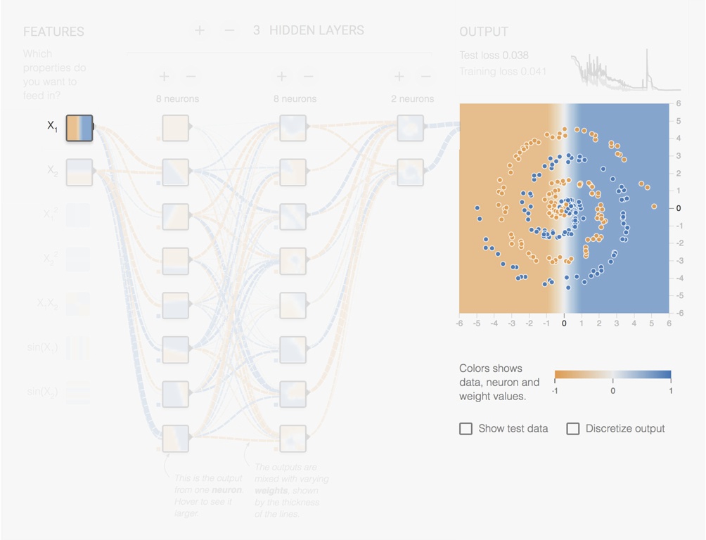
Figure 5.12: Screenshot from the Tensorflow Playground page.

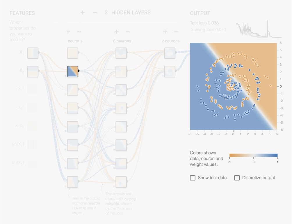
Figure 5.13: Screenshot from the Tensorflow Playground page. Output of one of the Layer 1 neurons.

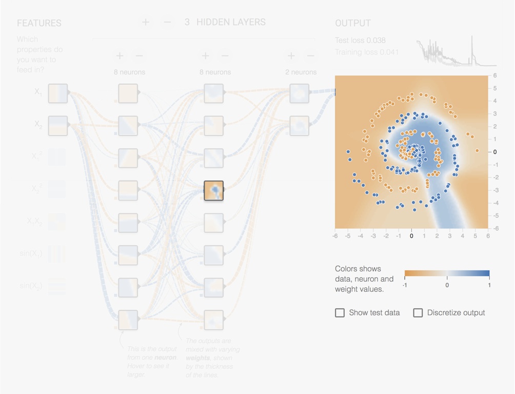
Figure 5.14: Screenshot from the Tensorflow Playground page. Output of one of the Layer 2 neurons.

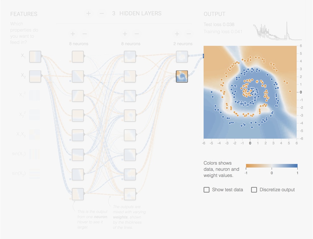
Figure 5.15: Screenshot from the Tensorflow Playground page. Output of one of the Layer 3 neurons.

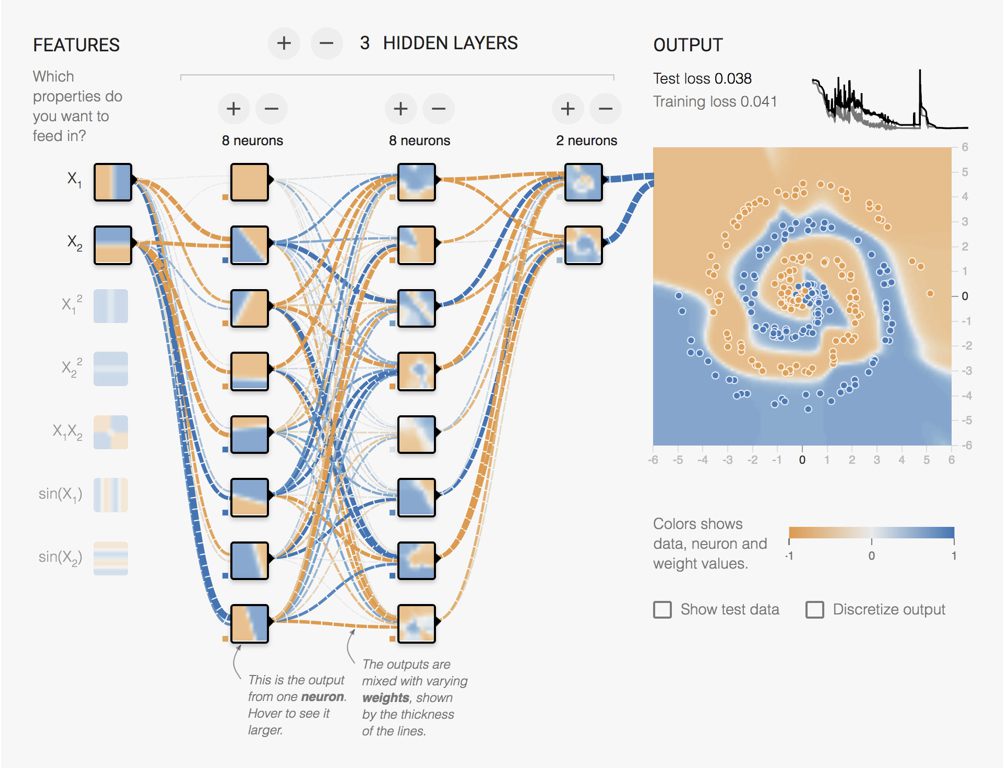
Figure 5.16: Screenshot from the Tensorflow Playground page. Output of the final unit.

One of the key properties of Neural Nets is their ability to learn how to build arbitrary complex features.

The deeper you go in the network, the more advanced the features are. Thus, even if deeper networks are harder to train, they tend to be more powerful and generalise better.

5.6 Training

At its core, a neural net evaluates a function $f$ of the input ${\bf x} = (x_1, \cdots, x_p)$ and weights ${\bf w} = (w_1, \cdots, w_q)$ and returns output values ${\bf y} = (y_1, \cdots, y_r)$:

\[ f(x_1, \cdots, x_p, w_1, \cdots, w_q) = (y_1,\cdots, y_r) \]

An example of the graph of operations for evaluating the model is presented next in Fig. 5.17. In this graph, the units are not neuron-types but simply some arbitrary functions. For instance we could have defined $u_7$ as $u_7: (u_1,u_2,u_3,u_4) \mapsto \cos(u_1+u_2+u_3)\exp(-2u_4)$ and $u_8$ as $u_8: (u_1,u_2,u_3,u_4) \mapsto \sin(u_1+u_2+u_3)\exp(-3u_4)$.

To show the universality of the graph representation, all inputs, weights and outputs values in this example have been renamed as $u_j$, where $j$ is the index of the corresponding unit. Thus, for an input feature vector ${\bf x}_i=[u_1,u_2,u_3]^{\top}$ and weights ${\bf w}=[u_4,u_5]^{\top}$, the output vector is $f({\bf x}_i, {\bf w})=[u_{12},u_{13},u_{14}]$.

Figure 5.17: Example of a graph of operations for neural net evaluation.

During training, we need to evaluate the output of $f({\bf x}_i, {\bf w})$ for a particular observation ${\bf x}_i$ and compare it to a observed result ${\bf y}_i$. This is done through a loss function $E$.

Typically the loss function aggregates results over all observations: \[ E({\bf w}) = \sum_{i=1}^n e(f({\bf x}_i, {\bf w}), {\bf y}_i), \] where $e(f({\bf x}_i, {\bf w}), {\bf y}_i)$ is the loss for an individual observation ${\bf x}_i$.

Thus we can build a graph of operations for training a single observation (see Fig. 5.18). It is the same graph as for evaluation but with all outputs units connected to a loss function unit.

Figure 5.18: Example of a graph of operations for neural net training.

To be precise, Fig 5.18 is the graph for a single observation. The complete training graph would combine all observations to compute the total loss $E$.

To optimise for the weights ${\bf w}$, we resort to a gradient descent approach. Starting from an initial state ${\bf w}^{(0)}$, we update the weights as follows:

\[ {\bf w}^{(m+1)} = {\bf w}^{(m)} - \eta \frac{\partial E}{\partial {\bf w}}({\bf w}^{(m)}) \] where $\frac{\partial E}{\partial {\bf w}}({\bf w}^{(m)}) = \sum_{i=1}^n \frac{\partial e}{\partial {\bf w}}({\bf w}^{(m)})(f({\bf x}_i, {\bf w}), {\bf y}_i)$ is the combined gradient over the dataset for the particular parameter values ${\bf w}^{(m)}$. The scalar $\eta$ is the learning rate which controls the speed of the descent (the higher the learning rate the faster the descent).

So we can train any neural net, as long as we know how to compute the gradient $\frac{\partial e}{\partial {\bf w}}({\bf w})$ for any particular set of parameters ${\bf w}$.

The Back Propagation algorithm will help us compute this gradient $\frac{\partial e}{\partial {\bf w}}({\bf w})$.

5.7 Back-Propagation

Backpropagation (backprop) was pioneered by David E. Rumelhart, Geoffrey E. Hinton, and Ronald J. Williams in 1986.

Rumelhart, David E., Geoffrey E. Hinton, and Ronald J. Williams. “Learning representations by back-propagating errors.” Cognitive Modeling 5.3 (1988): 1.

5.7.1 Computing the Gradient

What is the problem with computing the gradient?

Say we want to compute the partial derivative for a particular weight $w_{i}$. We could naively compute the gradient by numerical differentiation: \[ \frac{\partial e}{\partial w_{i}} \approx \frac{e(\cdots, w_{i}+\varepsilon, \cdots) - e(\cdots, w_{i}, \cdots)}{\varepsilon} \] with $\varepsilon$ sufficiently small. This is easy to code and quite fast.

Now, modern neural nets can easily have 100M parameters. Computing the gradient this way requires 100M evaluations of the network.

Not a good plan.

Back-Propagation will do it in about 2 passes.

Back-Propagation is the very algorithm that made neural nets a viable machine learning method.

To compute an output $y$ from an input ${\bf x}$ in a feedforward net, we process information forward through the graph, evaluate all hidden units $u$ and finally produces $y$. This is called forward propagation.

During training, forward propagation continues to produce a scalar error $e({\bf w})$.

The back-propagation algorithm then uses the Chain-Rule to propagate the gradient information from the cost unit back to the weights units.

5.7.2 The Chain Rule

Recall what the chain-rule is. Suppose you have a small graph, with a variable dependency as follows: $x \rightarrow y \rightarrow z$. Assuming $z=f(y)$ and $y=g(x)$ then we can compute the gradient $\frac{dz}{dx}$ by simply combining the intermediate gradients $\frac{dz}{dy}$ and $\frac{dy}{dx}$: \[ \frac{dz}{dx} = \frac{dz}{dy}\frac{dy}{dx} = f'(y)g'(x) = f'(g(x))g'(x) \]

In n-dimensions, things are a bit more complicated. Suppose that $z=f(u_1, \cdots, u_n)$, and that for $k=1,\dots,n$, $u_k=g_k(x)$. Then the chain-rule tells us that:

\[\begin{equation} \frac{\partial z}{\partial x} = \sum_k \frac{\partial z}{\partial u_k} \frac{\partial u_k}{\partial x} \end{equation}\]

Example 5.1 Assume that $u(x, y) = x^2 + y^2$, $y(r, t) = r \sin(t)$ and $x(r,t) = r \cos(t)$,

\[\begin{split} {\frac {\partial u}{\partial r}} &={\frac {\partial u}{\partial x}}{\frac {\partial x}{\partial r}}+{\frac {\partial u}{\partial y}}{\frac {\partial y}{\partial r}} \\ &=(2x)(\cos(t))+(2y)(\sin(t)) \\ &=2r(\sin ^{2}(t)+\cos^2(t))\\&= 2r \end{split} \]

5.7.3 Back-Propagating with the Chain-Rule

Let’s come back to our neural net example and let’s see how the chain-rule can be used to back-propagate the differentiation.

Figure 5.19: Backpropagation.

After the forward pass, we have evaluated all units $u$ and finished with the loss $e$.
We can evaluate the partial derivatives $\frac{\partial e}{\partial u_{14}}$, $\frac{\partial e}{\partial u_{13}}$, $\frac{\partial e}{\partial u_{12}}$ from the definition of $e$.

Remember that $e$ is simply a function of $u_{12}, u_{13}, u_{14}$.

For instance, if \[ e(u_{12},u_{13},u_{14}) = (u_{12}-a)^2 + (u_{13}-b)^2 + (u_{14}-c)^2, \] then \[ \frac{\partial e}{\partial u_{12}} = 2(u_{12} - a) \quad, \frac{\partial e}{\partial u_{13}} = 2(u_{13} - b) \quad, \frac{\partial e}{\partial u_{14}} = 2(u_{14} - c). \]

Figure 5.20: Backpropagation.

Now that we have computed $\frac{\partial e}{\partial u_{14}}$, $\frac{\partial e}{\partial u_{13}}$ and $\frac{\partial e}{\partial u_{12}}$, how do we compute $\frac{\partial e}{\partial u_{10}}$?

We can use the chain-rule: \[ \frac{\partial e}{\partial u_i} = \sum_{j \in \mathrm{Outputs}(i)} \frac{\partial u_j}{\partial u_i} \frac{\partial e}{\partial u_j} \] The Chain Rule links the gradient for $u_i$ to all of the $u_j$ that depend on $u_i$. In our case $u_{14}$, $u_{13}$ and $u_{12}$ depend on $u_{10}$. So the chain-rule tells us that: \[ \frac{\partial e}{\partial u_{10}} = \frac{\partial u_{14}}{\partial u_{10}} \frac{\partial e}{\partial u_{14}} + \frac{\partial u_{13}}{\partial u_{10}} \frac{\partial e}{\partial u_{13}} + \frac{\partial u_{12}}{\partial u_{10}} \frac{\partial e}{\partial u_{12}} \]

For instance if $u_{14}( u_5, u_{10}, u_{11}, u_{9}) = u_5 + 0.2 u_{10} + 0.7 u_{11} + 0.3 u_{9}$, then $\frac{\partial u_{14}}{\partial u_{10}}= 0.2$

We can now propagate back the computations and derive the gradient for each node at a time.

\[ \frac{\partial e}{\partial u_{9}} = \frac{\partial u_{14}}{\partial u_{9}} \frac{\partial e}{\partial u_{14}} + \frac{\partial u_{13}}{\partial u_{9}} \frac{\partial e}{\partial u_{13}} + \frac{\partial u_{12}}{\partial u_{9}} \frac{\partial e}{\partial u_{12}} \]

\[ \frac{\partial e}{\partial u_{11}} = \frac{\partial u_{14}}{\partial u_{11}} \frac{\partial e}{\partial u_{14}} + \frac{\partial u_{13}}{\partial u_{11}} \frac{\partial e}{\partial u_{13}} + \frac{\partial u_{12}}{\partial u_{11}} \frac{\partial e}{\partial u_{12}} \]

\[ \begin{split} \frac{\partial e}{\partial u_{5}} = & \frac{\partial u_{14}}{\partial u_{5}} \frac{\partial e}{\partial u_{14}} + \frac{\partial u_{13}}{\partial u_{5}} \frac{\partial e}{\partial u_{13}} + \frac{\partial u_{12}}{\partial u_{5}} \frac{\partial e}{\partial u_{12}} \\ & + \frac{\partial u_{11}}{\partial u_{5}} \frac{\partial e}{\partial u_{11}} + \frac{\partial u_{10}}{\partial u_{5}} \frac{\partial e}{\partial u_{10}} + \frac{\partial u_{9}}{\partial u_{5}} \frac{\partial e}{\partial u_{9}} \end{split} \]

\[ \frac{\partial e}{\partial u_{6}} = \frac{\partial u_{14}}{\partial u_{6}} \frac{\partial e}{\partial u_{14}} + \frac{\partial u_{13}}{\partial u_{6}} \frac{\partial e}{\partial u_{13}} + \frac{\partial u_{12}}{\partial u_{6}} \frac{\partial e}{\partial u_{12}} \]

\[ \begin{split} \frac{\partial e}{\partial u_{4}} = & \frac{\partial u_{8}}{\partial u_{4}} \frac{\partial e}{\partial u_{8}} + \frac{\partial u_{7}}{\partial u_{4}} \frac{\partial e}{\partial u_{7}} + \frac{\partial u_{6}}{\partial u_{4}} \frac{\partial e}{\partial u_{6}} \\ & + \frac{\partial u_{11}}{\partial u_{4}} \frac{\partial e}{\partial u_{11}} + \frac{\partial u_{10}}{\partial u_{4}} \frac{\partial e}{\partial u_{10}} + \frac{\partial u_{9}}{\partial u_{4}} \frac{\partial e}{\partial u_{9}} \end{split} \]

Figure 5.21: Backpropagation.

Figure 5.22: Backpropagation.

As you can see Back Propagation proceeds by induction. Assume that we know how to compute $\frac{\partial E}{\partial u_j}$ for a subset of units $\mathcal{K}$ of the network. Pick a node $i$ outside of $\mathcal{K}$ but with all of its outputs in $\mathcal{K}$. We can compute $\frac{\partial e}{\partial u_i}$ using the chain-rule:

\[\begin{eqnarray*} \frac{\partial e}{\partial u_i} &=& \sum_{j \in \mathrm{Outputs}(i) } \frac{\partial e}{\partial u_j} \frac{\partial u_j}{\partial u_i} \end{eqnarray*}\]

As we already have computed $\frac{\partial e}{\partial u_j}$ for $j \in \mathcal{K}$ and we can now directly compute $\frac{\partial u_j}{\partial u_i}$ by differentiating the function $u_j$ with respect to its input $u_i$.

We can stop the back propagation once $\frac{\partial e}{\partial u_i}$ has been computed for all the parameter units in the graph.

Back-Propagation is the fastest method we have to compute the gradient in a graph.

The worst case complexity of backprop is $\mathcal{O}(\mathrm{number\_of\_units}^2)$ but in practice for most network architectures it is $\mathcal{O}(\mathrm{number\_of\_units})$.

Back-Propagation is what makes training deep neural nets possible.

5.7.4 Vanishing Gradients

One major challenge when training deeper networks is the problem of vanishing gradients.

Hochreiter, S. (1991). Untersuchungen zu dynamischen neuronalen Netzen (PDF) (diploma thesis). Technical University Munich, Institute of Computer Science.

Consider training the following deep network with 6 hidden layers:

Figure 5.23: Backpropagation.

The gradient $\frac{de}{dw}$ is as follows: \[ \frac{de}{dw} = \frac{de}{du_6}\frac{du_6}{du_5}\frac{du_5}{du_4}\frac{du_4}{du_3}\frac{du_3}{du_2}\frac{du_2}{du_1}\frac{du_1}{dw} \] It is a product, so if any of $\left|\frac{de}{du_6}\right|, \dots, \left|\frac{du_1}{dw}\right|$ is near zero, then the resulting gradient will also be near zero.

In Fig. 5.24, Fig. 5.25 and Fig. 5.26 are shown the derivatives of some popular activation functions.

Figure 5.24: Derivative of the sigmoid activation function.

Figure 5.25: Derivative of the tanh activation function.

Figure 5.26: Derivative of the ReLu activation function.

For most of the input range (eg. outside [-5, 5]), the values of the derivatives are zero or near zero. There is thus a great risk for at least one of the units to produce a near zero derivative. When this happens we have $\frac{de}{dw}\approx 0$ and the gradient descent will get stuck.

The problem of vanishing gradients is a key difficulty when training Deep Neural Networks. It is also one of the reasons ReLU is sometimes preferred as at least half of the range has a non-null gradient.

Recent modern network architectures try to mitigate this problem (see ResNets and LSTM).

5.8 Optimisations for Training Deep Neural Networks

We have seen how weights can be trained through a gradient descent algorithm and how the gradient at each step can be computed via the Back-Propagation algorithm.

The problem that is now faced by all deep learning practitioners is that gradient descent approaches are not guaranteed to converge to a global minimum, nor to a local minimum in fact.

Tuning the training optimisation will thus be a critical task when developing neural networks applications. There are no secret sauce to find the right combination of hyper parameters and many trials and errors may be required.

A few optimisation strategies and regularisation techniques are however available to help with the convergence.

5.8.1 Mini-Batch and Stochastic Gradient Descent

Recall the gradient descent step:

\[ {\bf w}^{(m+1)} = {\bf w}^{(m)} - \eta \frac{\partial E}{\partial {\bf w}}({\bf w}^{(m)}) \]

The loss function is usually constructed as the average error for all observations:

\[ E({\bf w}) = \frac{1}{n} \sum_{i=1}^n e(f({\bf x}_i, {\bf w}), {\bf y}_i) \]

We’ve seen how to compute $\frac{\partial e}{\partial {\bf w}}$ for a particular observation ${\bf x}_i$ using backpropagation. The combined gradient for $E$ is simply:

\[ \frac{\partial E}{\partial {\bf w}} = \frac{1}{n} \sum_{i=1}^n \frac{\partial e}{\partial {\bf w}} (f({\bf x}_i, {\bf w}), {\bf y}_i) \]

This requires evaluating the gradient for the entire dataset, which is usually not practical.

A very common approach is instead to compute the gradient over batches of the training data. For instance if the batch size is 16, that means that the gradient used in the gradient descend algorithm is only averaged over 16 observations. For instance, starting from observation $j$:

\[ \frac{\partial E}{\partial {\bf w}} \approx \frac{1}{16} \sum_{i=j}^{j+15} \frac{\partial e}{\partial {\bf w}} (f({\bf x}_i, {\bf w}), {\bf y}_i) \]

Next evaluation of the gradient starts at $j+16$.

This process is called mini-batch gradient descent.

In the edge case where the batch size is 1, the gradient is recomputed for each observation:

\[ \frac{\partial E}{\partial {\bf w}} \approx \frac{\partial e}{\partial {\bf w}} (f({\bf x}_i, {\bf w}), {\bf y}_i) \]

and the process is called Stochastic Gradient Descent (SGD)

The smaller the batch size, the faster a step of the gradient descent can be done. Small batch sizes also mean that the computed gradient is a bit “noisier”, and likely to change from batch to batch. This randomness can help escape from local minimums but can also lead to poor convergence.

An epoch is a measure of the number of times all of the training vectors are used once to update the weights.

After one epoch, the gradient descent will have done $n$/BatchSize steps.

Note that after each epoch the samples are usually shuffled so as to avoid cyclical repetitions.

5.8.2 More Advanced Gradient Descent Optimizers

Sometimes the vanilla gradient descent is not the most efficient way. In this example the loss function forms a deep and long valley. In this scenario the gradient descent is not very efficient at reaching the minimum.

Figure 5.27: Illustration of a Stochastic Gradient Descent.

In particular, we can observe that the steepest descent of the gradient can take many changes of direction.

One technique to reduce that problem is to cool down —or decay— the learning rate over time.

Another approach is to reuse previous gradients to influence the current update. For instance, the momentum update technique tries to average out the gradient direction over time as follows: \[\begin{align*} {\bf v}^{(m+1)} &= \mu {\bf v}^{(m)} - \eta \frac{\partial E}{\partial {\bf w}}({\bf w}^{(m)}) \\ {\bf w}^{(m+1)} &= {\bf w}^{(m)} + {\bf v}^{(m+1)} \end{align*}\] with $\mu\approx 0.9$

Other more sophisticated techniques exist. To name of few:

Nesterov Momentum, Nesterov’s Accelerated Momentum (NAG), Adagrad, RMSprop, Adam and Nadam.

Adam and Nadam are known to usually perform best but this may change depending on your problem. So it’s okay to try a few out.

http://cs231n.github.io/neural-networks-3/

5.9 Constraints and Regularisers

5.9.1 L2 regularisation

L2 is the most common form of regularisation. It is the Tikhonov regularisation of Least Squares. To add a L2 regularisation on a particular weight $w_i$, we simply add a penalty to the loss function:

\[ E'({\bf w}) = E({\bf w}) + \lambda w_i^2 \]

5.9.2 L1 regularisation

L1 is another common form of regularisation:

\[ E'({\bf w}) = E({\bf w}) + \lambda |w_i| \]

L1 regularisation can have the desirable effect of settings weights $w_i$ to zero and thus simplifying the network (see note A.2).

https://keras.io/api/layers/regularization_layers/

5.10 Dropout & Noise

We know that one way of fighting overfitting is to use more data.

One cheap way to obtain more data is to take the original observations and add a bit of random noise to the features. This can be done synthetically by adding noise to the original dataset (eg. adding Gaussian noise to the original features).

One step further is to add noise, during the training phase, to the hidden units themselves.

https://keras.io/api/layers/regularization_layers/gaussian_noise/

With Dropout, units are randomly switched off during training (ie. the randomly selected units have their output set to zero).

Dropout can be seen as applying a multiplicative binary noise to the layers.

https://keras.io/api/layers/regularization_layers/dropout/

5.11 Monitoring and Training Diagnostics

Training can take a long time. From an hour to a few days. You need to carefully monitor the loss function during training. The more information you track, the easier it is to diagnostic your training.

Similarly to what we saw with logistic regression, the trend of the loss function during training can tell us whether the learning rate is suitable. If the learning rate is too high, the gradient descent might overshoot local minima or diverge drastically (see Figure 5.28). If the learning rate is too low, the training will take too long to be of practical use.

Figure 5.28: Possible effects of the Learning Rate on the training.

Also, remember from Least Squares that good performance in training and poor performance in testing/validation is a sign of overfitting. See Figure 5.29 for some examples.

Figure 5.29: Detecting Overfitting in Training.

5.12 Take Away

You can see Deep Neural Networks as a framework to model any function as a network of basic units (the neurons).

The universal approximation theorem guarantees us that any function can indeed be approximated this way.

How to best architect the networks is main research question today. Deeper networks are known to be more efficient but harder to train because of the problem of vanishing gradients.

Training the weights of the network can be done through a gradient descent algorithm. The gradient at each step can be computed via the Back-Propagation algorithm.

Gradient descent approaches are however not guaranteed to converge to a global minimum. We must thus carefully monitor the optimisation. A few optimisation strategies and regularisation techniques are available to help with the convergence. Training networks requires a lot of trial and error.

5.13 Useful Resources

[1] Deep Learning (MIT press) from Ian Goodfellow et al. - chapters 6, 7 & 8, https://www.deeplearningbook.org

[2] Brandon Rohrer YT channel, https://youtu.be/ILsA4nyG7I0

[3] 3Blue1Brown YT video, https://youtu.be/aircAruvnKk

[4] 3Blue1Brown YT video, https://youtu.be/IHZwWFHWa-w

[5] Stanford CS class CS231n, http://cs231n.github.io

[6] Tensorflow playground, https://playground.tensorflow.org

[7] Michael Nielsen’s webpage, http://neuralnetworksanddeeplearning.com/