Chapter 7 Advances in Network Architectures
In this chapter are covered some of the important advances in network architectures between 2012 and 2015.
These advances try to address some of the major difficulties in DNN’s, including the problem of vanishing gradients when training deeper networks. The idea is to try to highlight some of the typical components of a modern architecture and training pipeline.
7.1 Transfer Learning
7.1.1 Re-Using Pre-Trained Networks
Transfer learning is the idea of reusing knowledge learned from a task to boost performance on a related task.
Say you are asked to develop a DNN application that can recognise pelicans on images. Training a state of the art CNN network from scratch can necessitate weeks of training and hundreds of thousands of pictures. This would be unpractical in your case because you can only source a thousand images.
What can you do? You can reuse parts of existing networks.
Recall the architecture of AlexNet (2012) in Fig. 7.1.
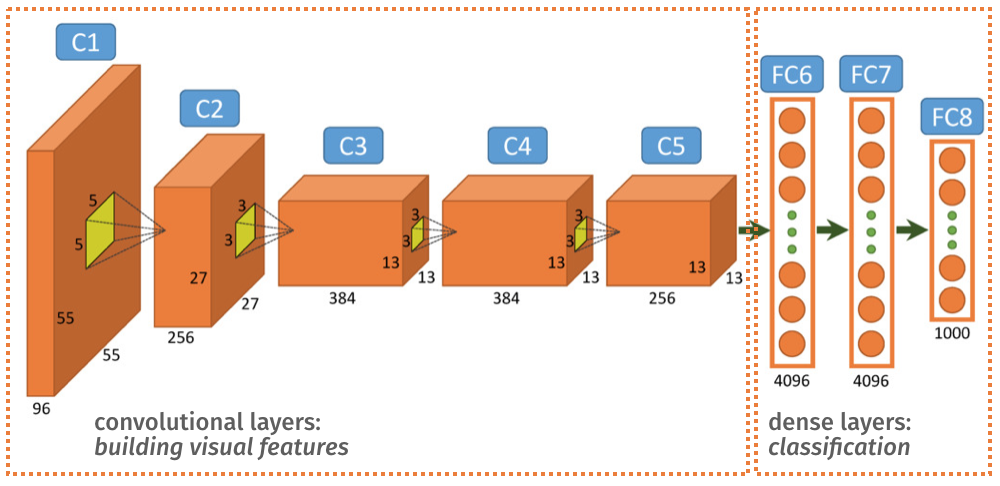
Figure 7.1: AlexNet
Broadly speaking the convolutional layers (up to C5) build visual features whilst the last dense layers (FC6, FC7 and FC8) perform classification based on these visual features.
AlexNet (and any of the popular off-the-shelf networks such as VGG, ResNet or GoogLeNet) was trained on millions of images and thousands of classes. The network is thus able to deal with a great variety of problems and the trained filters produce very generic features that are relevant to most visual applications.
Therefore AlexNet’s visual features could be very effective for your particular task and maybe there is no need to train new visual features: just reuse these existing ones.
The only task left is to design and train the classification part of the network (eg. the dense layers).
Your application looks like this: copy/paste a pre-trained network, cut away the last few layers and replace them with your own specialised network.
Depending on the amount of training data available to you, you may decide to only redesign the last layer (ie. FC8), or a handful of layers (eg. C5, FC6, FC7, FC8). Keep in mind that redesigning more layers will necessitate more training data.
If you have enough samples, you might want to allow backpropagation to update some of the imported layers, so as to fine tune the features for your specific application. If you don’t have enough data, you probably should freeze the values of the imported weights.
In Keras you can freeze the update of parameters using the trainable=False argument. For instance:
In most image based applications you should first consider reusing off-the-shelf networks such as VGG, GoogLeNet or ResNet. It has been shown (see link below) that using such generic visual features yield state of the art performances in most applications.
Razavian et al. ``CNN Features off-the-shelf: an Astounding Baseline for Recognition’’. 2014. https://arxiv.org/abs/1403.6382
7.1.2 Domain Adaption and Vanishing Gradients
Let’s see why re-using networks on new training sets can be difficult. Consider a single neuron and assume a \(\mathrm{tanh}\) activation function \(f(x_i, w) = \mathrm{tanh}(x_i+w)\). The training samples shown in Fig.7.2 are images taken on a sunny day. The input values \(x_i\) (red dots) are centred about \(0\) and the estimated \(w\) is \(\hat{w}=0\).

Figure 7.2: Domain Shift Example.
We want to fine tune the training with new images taken on cloudy days. The new samples values \(x_i\) (green crosses) are centred around \(5\). For that input range, the derivative of \(\mathrm{tanh}\) is almost zero, which means we have a problem of vanishing gradients. It will be difficult to update the network weights.
7.1.3 Normalisation Layers
It is thus critical for the input data to be in the correct value range. To cope with possible shifts of value range between datasets we can use a Normalisation Layer, whose purpose it to scale the data according to the training set statistics.
Denoting \(x_{i}\) an input value of the normalisation layer, the output \(x_i'\) after normalisation is defined as follows:
\[ x'_{i} = \frac{x_{i} - \mu_i}{\sigma_i} \]
where \(\mu_i\) and \(\sigma_i\) are computed off-line based on the input data statistics.
The samples after normalisation are shown in Fig.7.3.

Figure 7.3: Domain Shift After Normalisation.
7.1.4 Batch Normalisation
Batch Normalisation (BN) is a particular type of normalisation layer where the rescaling parameters \(\mu\) and \(\sigma\) are chosen as follows.
For training, \(\mu_i\) and \(\sigma_i\) are set as the mean value and standard deviation of \(x_i\) over the mini-batch. That way the distribution of the values of \(x_i'\) after BN is 0 centred and with variance 1.
For evaluation, \(\mu_i\) and \(\sigma_i\) are averaged over the entire training set.
BN can help to achieve higher learning rates and be less careful about optimisation considerations such as initialisation or Dropout.
Sergey Ioffe, Christian Szegedy. “Batch Normalization: Accelerating Deep Network Training by Reducing Internal Covariate Shift.” (2015) https://arxiv.org/abs/1502.03167
7.2 Going Deeper
As the potential for deeper networks to generalise better became evident, a fervent competition to push the boundaries further began after 2012.
The key hurdle in this race was that, because of vanishing gradients, sequential architectures like VGG couldn’t be trained for more than 14-16 layers.
Recall the problem of vanishing gradients on this simple network:

\[ \frac{\partial e}{\partial w} = \frac{\partial e}{\partial u_2} \frac{\partial u_2}{\partial u_1} \frac{\partial u_1}{\partial w} \]
During the gradient descent, we evaluate \(\frac{\partial e}{\partial w}\), which is a product of the intermediate derivatives. If any of these is zero, then \(\frac{\partial e}{\partial w}\approx 0\).
Now consider the layer containing \(u_2\), and replace it with a network of 3 units in parallel (\(u_3\), \(u_2\), \(u_4\)).

\[ \frac{\partial e}{\partial w} = \frac{\partial e}{\partial u_2} \frac{\partial u_2}{\partial u_1} \frac{\partial u_1}{\partial w} \color{gRed} + \frac{\partial e}{\partial u_4} \frac{\partial u_4}{\partial u_1} \frac{\partial u_1}{\partial w} + \frac{\partial e}{\partial u_3} \frac{\partial u_3}{\partial u_1} \frac{\partial u_1}{\partial w} \]
It is now less likely to \(\frac{\partial e}{\partial w}\approx 0\) as all three terms need to be null.
So a simple way of mitigating vanishing gradients is to avoid a pure sequential architecture and introduce parallel paths in the network.
This is what was proposed in GoogLeNet (2014) and ResNet (2015).
7.2.1 GoogLeNet: Inception
GoogLeNet was the winner of ILSVRC 2014 (the annual competition on ImageNet) with a top 5 error rate of 6.7% (human error rate is around 5%).
The CNN is 22 layer deep (compared to the 16 layers of VGG).
Szegedy et al. “Going Deeper with Convolutions”, \ CVPR 2015. (paper link: https://goo.gl/QTCe66)
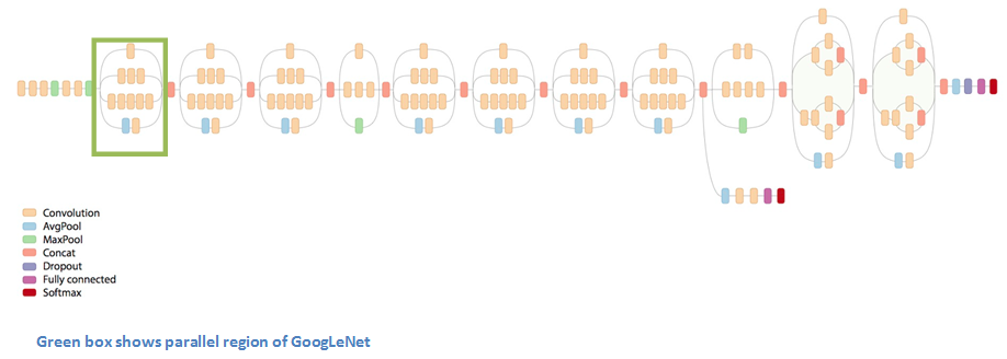
Figure 7.4: GoogLeNet
The architecture resembles the one of VGG, except that instead of a sequence of convolution layers, we have a sequence of inception layers (eg. green box).
An inception layer is a sub-network (hence the name inception) that produces 4 different types of convolutions filters, which are then concatenated (see this video: https://youtu.be/VxhSouuSZDY).
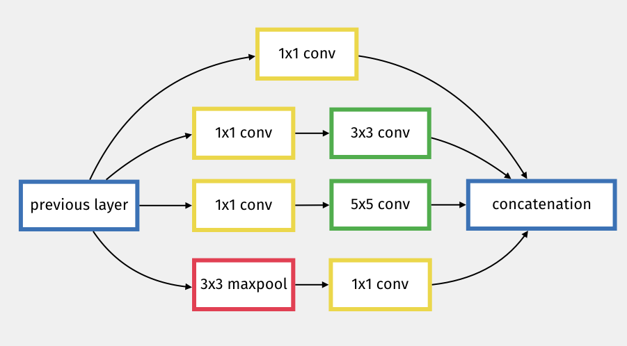
Figure 7.5: GoogLeNet Inception Sub-Network
The inception network creates parallel paths that help with the vanishing gradient problem and allow for a deeper architecture.
7.2.2 ResNet: Residual Network
ResNet is a 152 (yes, 152!!) layer network architecture developed at Microsoft Research that won ILSVRC 2015 with an error rate of 3.6% (better than human performance).
Kaiming He et al (2015). “Deep Residual Learning for Image Recognition”. https://goo.gl/Zs6G6X
Similarly to GoogLeNet, at the heart of ResNet is the idea of creating parallel connections between deeper layers and shallower layers. The connection is simply done by adding the result of a previous layer to the result after 2 convolutions layers:
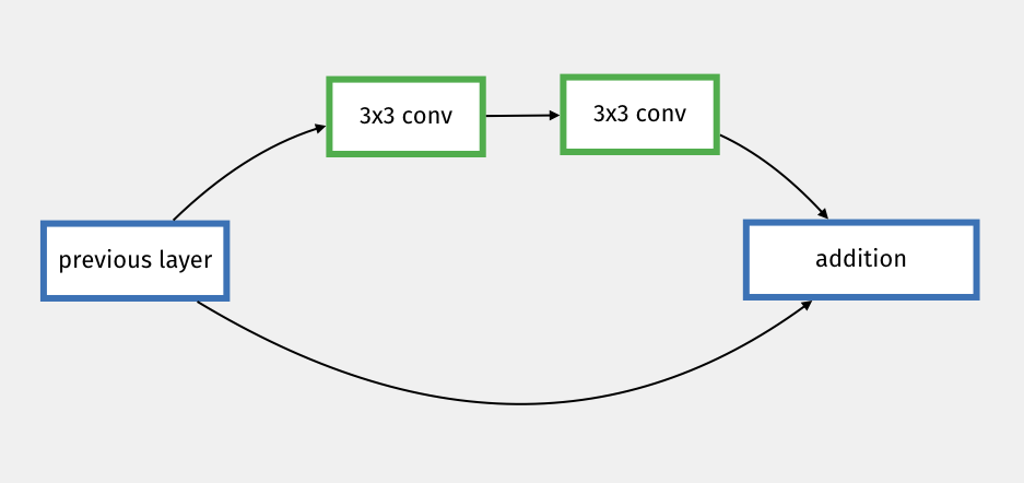
Figure 7.6: ResNet Sub-Network
The idea is very simple but allows for a very deep and very efficient architecture.
The ResNet architecture has been hugely successful. Many ResNet variants, pre-trained on ImageNet, can be found, such as the ResNet-18/34/50/101/151 models.
7.3 A Modern Training Pipeline
7.3.1 Data Augmentation
It is often possible to naturally increase your dataset by generating variants of your input data.
For instance, with images, we know that minor image processing operations, such as crop, flip, rotation, zoom, contrast change, JPEG compression, noise, etc. should not change the outcome.
Therefore these variants allow us to expand our dataset for free.
see https://keras.io/api/layers/preprocessing_layers/image_augmentation/
Similar ideas can be applied in other domains. For instance, in audio, you can also add noise, compression, reverb, etc.
Sometimes a good way to get data is to synthesise data through a similuation model (e.g. using game engine). Be mindful, however, that this artificial data is a simplified model of the real-world problem, and thus can lead to overfitting. Also, synthetic data tends to have slightly different characteristics from real data, and we will need to be careful with domain adaptation issues.
Generative DNNs (see later chapter) can also be used to sytnthesise data (e.g. you can use ChatGTP to generate text for your dataset, or dialogue interactions for your bots).
7.3.2 Initialisation
Initialisation needs to be considered carefully. Starting at \(w=0\) is probably not a good idea, as you are likely to be stuck into some special local minimum, with the gradient being zero right from the start.
The idea would then be to start at random. We need, however to be careful, and control the output at each layer to avoid a situation where gradients would explode or vanish through the different layers.
For ReLU, a popular initialisation is He’s initialisation. For each layer \(l\), the bias \(b\) and weights \(w\) are initialised as \(b_l=0, w_l\sim \mathcal{N}(0, \sqrt{2/n_{l-1}})\), where \(n_{l-1}\) is the number of neurons in prev layer. Using this guarantees stable gradients throughout the network (at least at the start of the training).
More Detailed Explanations and very nice Demos https://www.deeplearning.ai/ai-notes/initialization/
Kaiming He et al. Delving Deep into Rectifiers https://arxiv.org/abs/1502.01852
Here is a quick overview of how this works (non-examinable material).
Consider a sequence of conv or dense layers (indexed \(l\)). The logits and ReLU activations can be derived as follows: \[ {\bf y}_l = {\bf W}_l {\bf x}_l \quad \text{and} \quad {\bf x}_l = \max({\bf y}_{l-1},0). \]
Assuming independence and weights and biases with zero mean:
\[ \mathrm{Var}[y_l] = n_l \mathrm{Var}[w_lx_l] = n_l \mathrm{Var}[w_l]E[x_l^2]. \]
For ReLU, \(x_l =0\) for \(y_{l-1} < 0\), thus \(E[x_l^2] = \frac{1}{2}\mathrm{Var}[y_{l-1}]\), and
\[ \mathrm{Var}[y_l] = \frac{1}{2}n_l \mathrm{Var}[w_l] \mathrm{Var}[y_{l-1}]. \]
One way to avoid an increase/decrease of the variance throughout the layers is to set: \[ \mathrm{Var}[w_l] = \frac{2}{n_l}, \] which we can achieve by sampling \(w_l\) from \(\mathcal{N}(0, \sqrt{2/n_l})\).
7.3.3 Optimisation
As we have seen in previous chapters, a number of optimisation techniques are available to us for training. Papers in the literature tend to gravitate around Adam or SGD. Adam seems to be the fastest out of the box, but best-in-class models tend to be trained on SGD with momentum, as they find local minima that generalise better than the ones found by Adam.
Since then, an improved version of Adam, AdamW, was proposed and seems to fix Adam’s shortcomings.
Another aspect of the optimisation is the scheduling of the learning rate. We know that we should probably reduced the learning rate as we approach the local minimum.
In 2017 was popularised the idea of warm restarts, which periodically raise the learning rate to temporary diverge and allow to hop over hills. A variant of this scheme is the cosine annealing schedule:

Figure 7.7: AlexNet
An example of a reasonably modern optimiser scheme would look like this in Keras:
7.3.4 Take Away
It is typical for modern convolution networks to enhance the original convolution/activation block with a combination of normalisation layers and residual connections. The new blocks are much more resilient to the vanishing gradient problem, and allows both 1) to go much deeper, and 2) to be efficiently used for transfer learning.
Modern training pipelines typically include some data augmentation step, a dedicated initialisation strategy (eg. He or Xavier), a careful consideration of the optimisation (eg. AdamW) and of the learning rate schedule (eg. cosine annealing), with sometimes a transfer-learning/fine-tuning approach to kick start the training.
Keep in mind that there are no universal truth here. These are popular techniques but they might not be optimal for your problem.