9 An Introduction to Generative Models
Until now, our focus has primarily been on discriminative models. These models are trained to learn the boundary between different classes of data. Their goal is to estimate the conditional probability P(Y | X): given an input X, what is the probability of the label Y? Logistic regression, SVMs, and standard feed-forward classifiers are all examples of discriminative models. They are the workhorses of supervised learning, where we learn from a dataset of inputs {\bf X} that have been explicitly paired with ground-truth labels {\bf y}.
A Discriminative Task: Given a dataset of images labelled as either ‘face’ or ‘not face’, train a model to detect whether a new image contains a face.
In this chapter, we shift our focus to a different paradigm: generative models. Instead of learning to distinguish between classes, generative models aim to learn the underlying probability distribution of the data itself. Their goal is to model P(X) (the distribution of the data) or P(X | Y) (the distribution of data belonging to a specific class). The ultimate objective is to synthesise new data that is statistically similar to the data the model was trained on.
Because the goal is to learn the inherent structure of the data without relying on explicit labels, generative modelling is often a form of unsupervised learning.
A Generative Task: Given a large dataset of human faces, train a model that can generate new, realistic-looking faces of people who do not exist.
Deep learning has given rise to several powerful families of generative models, including:
- Generative Adversarial Networks (GANs)
- Autoencoders (AEs) and Variational Autoencoders (VAEs)
- Auto-Regressive Models (e.g., GPT-3, GPT-4)
- Diffusion Models (the technology behind popular image generation tools like Midjourney and DALL-E)
In this module, we will provide an introduction to GANs, Autoencoders, and Auto-Regressive Models.
9.1 Generative Adversarial Networks (GANs)
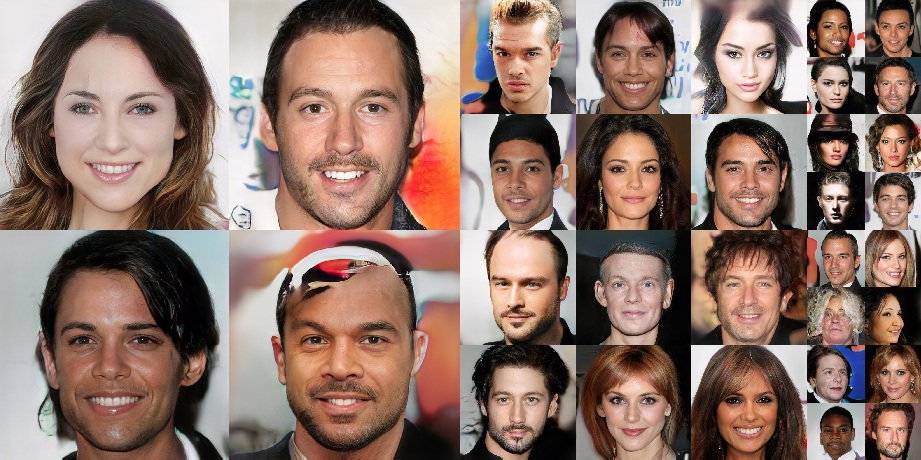
For several years, Generative Adversarial Networks were the dominant force in generative modelling, producing stunningly realistic images. The core idea, introduced by Ian Goodfellow and his colleagues in 2014, is both elegant and powerful. It frames the learning process as a two-player game.
Ian Goodfellow et al. (2014). “Generative Adversarial Networks”. https://arxiv.org/abs/1406.2661
A GAN consists of two neural networks that are trained in opposition to one another:
The Generator (G): Its job is to create fake data. It takes a random noise vector (a ‘seed’) as input and tries to transform it into a sample that looks like it could have come from the real dataset.
The Discriminator (D): Its job is to be a detective. It is a standard binary classifier that takes a sample (either a real one from the training set or a fake one from the generator) and must determine whether it is real or fake.
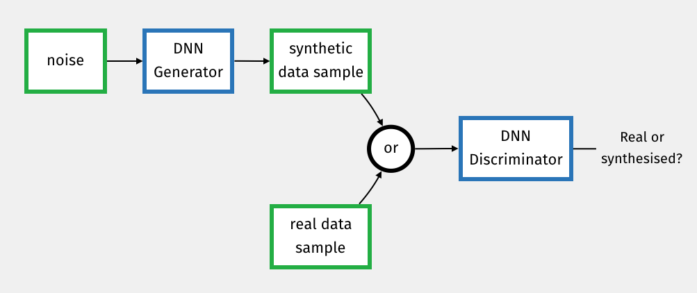
The training process is an adversarial game:
- The Generator wants to fool the Discriminator. Its loss is low when the Discriminator incorrectly classifies its fake images as real. So, it learns to produce increasingly realistic images.
- The Discriminator wants to correctly identify the fakes. Its loss is low when it correctly distinguishes between real and fake images. As the Generator gets better, the Discriminator must learn to spot ever more subtle flaws.
This creates an arms race. The Generator and Discriminator are trained alternately. A better Discriminator provides a more informative loss signal for the Generator, pushing it to create better fakes. In turn, a better Generator provides more challenging training data for the Discriminator. When this process reaches equilibrium, the Generator is producing samples that are so realistic that the Discriminator can do no better than random guessing.
Training GANs is notoriously difficult and unstable, but the results can be spectacular. They have been used to generate hyper-realistic images, artwork, and even music.
9.2 Autoencoders: Learning to Compress and Reconstruct
Autoencoders are a form of unsupervised learning where the learning signal comes from the data itself. The goal is simple: train a network to reconstruct its own input as faithfully as possible. While this sounds like a trivial task (the identity function would solve it perfectly), the key is that we force the data to pass through a bottleneck layer with a much lower dimensionality than the input.
An autoencoder consists of two parts:
- The Encoder: This part of the network takes the high-dimensional input data {\bf x} and compresses it into a low-dimensional latent representation {\bf z}.
- The Decoder: This part takes the latent representation {\bf z} and attempts to reconstruct the original input data, producing {\bf \hat{x}}.

The network is trained to minimise a reconstruction loss, which measures the difference between the original input {\bf x} and the reconstructed output {\bf \hat{x}}. For continuous data like images, this is typically the Mean Squared Error (L2 loss). For categorical data, it would be the cross-entropy loss.
By forcing the network to squeeze all the necessary information through the low-dimensional bottleneck, we compel it to learn a meaningful, compressed representation of the data. This process is a form of non-linear dimensionality reduction, similar in spirit to Principal Component Analysis (PCA).
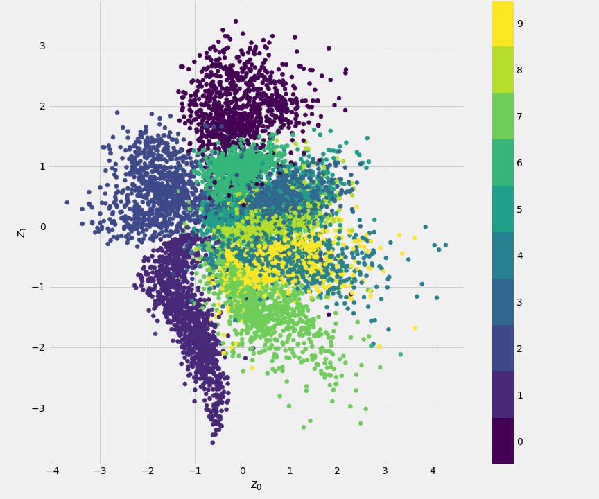
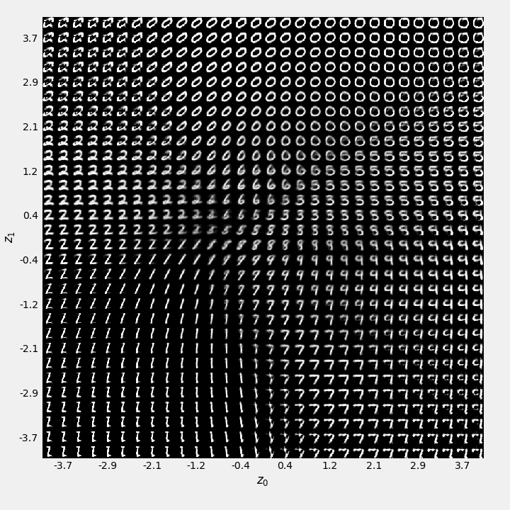
9.2.1 The Problem of the Latent Space
While autoencoders are excellent for tasks like denoising or dimensionality reduction, they are not inherently good generative models. The reason lies in the structure of the latent space—the space of all possible latent vectors {\bf z}.
A standard autoencoder makes no guarantees about the structure of this space. The encoder might learn to map input images to disconnected clusters in the latent space, with large gaps in between. If we were to pick a point {\bf z} from one of these gaps and feed it to the decoder, the resulting reconstruction {\bf \hat{x}} would likely be a blurry, meaningless mess, because the decoder was never trained on such a point.
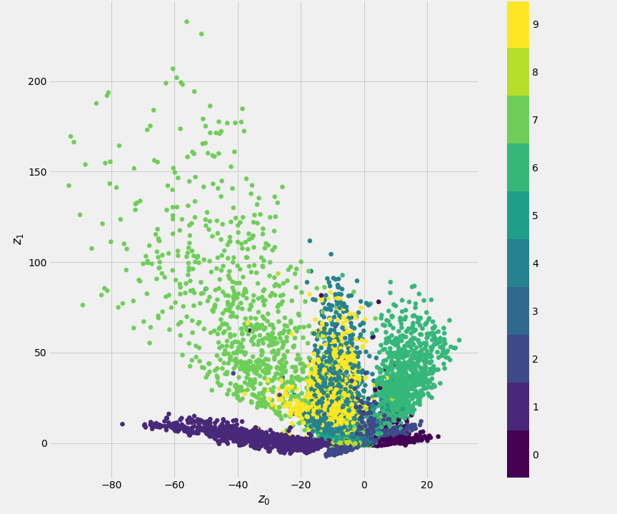
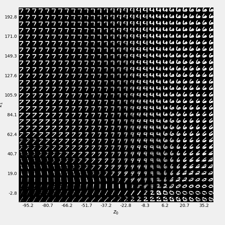
To build a true generative model, we need a latent space that is smooth, continuous, and well-structured, so that we can sample any point {\bf z} and be confident that the decoder will produce a valid output. This is the problem that Variational Autoencoders were designed to solve.
9.2.2 Variational Autoencoders (VAEs)
Variational Autoencoders (VAEs) are a more sophisticated type of autoencoder that makes them suitable for generation. They do this by introducing a probabilistic spin on the encoder and adding a new term to the loss function that enforces a regular structure on the latent space.
Instead of mapping an input {\bf x} to a single point {\bf z} in the latent space, the VAE encoder maps it to a probability distribution— specifically, a Gaussian distribution defined by a mean vector \boldsymbol{\mu} and a variance vector \boldsymbol{\sigma}^2. The latent vector {\bf z} is then sampled from this distribution.

The VAE loss function has two components:
The Reconstruction Loss: This is the same as in a standard AE. It pushes the model to accurately reconstruct the input.
The Kullback-Leibler (KL) Divergence Loss: This is the key addition. It measures how much the distribution produced by the encoder (\mathcal{N}(\boldsymbol{\mu},\boldsymbol{\sigma}^2)) differs from a standard normal distribution (\mathcal{N}(\mathbf{0},\mathbf{I})). This loss term acts as a regulariser, forcing the encoder to learn distributions that are centred around the origin and have unit variance. This ensures that the latent space is continuous and densely packed, without the gaps we saw in the standard AE.
By balancing these two losses, the VAE learns a smooth, structured latent space that is ideal for generation. To create a new sample, we no longer need an input image. We simply sample a random point {\bf z} from the standard normal distribution (\mathcal{N}(\mathbf{0}, \mathbf{I})) and pass it to the decoder.
9.3 Deep Auto-Regressive Models
Auto-regressive models are another powerful class of generative models that we have already encountered in the context of RNNs. The core idea is to model the probability distribution of a sequence by decomposing it using the chain rule of probability. The probability of a given element in the sequence is conditioned on all the elements that came before it:
\begin{equation} p(x_1, \dots, x_T) = \prod_{t=1}^T p(x_t | x_1, \dots, x_{t-1}) \end{equation}
This is exactly the principle behind character-level RNNs and the massive Large Language Models (LLMs) like GPT-3 and GPT-4. They are trained to predict p(x_t | x_1, \dots, x_{t-1}), the probability of the next word (or token) in a sequence given the preceding context.
By repeatedly sampling from the model’s predicted distribution and feeding the result back as input, they can generate coherent and sophisticated text, one token at a time.
9.4 Takeaways
Generative models learn the underlying distribution of a dataset in order to synthesise new data.
Generative Adversarial Networks (GANs) use a two-player game between a Generator and a Discriminator to produce highly realistic samples.
Autoencoders (AEs) are unsupervised models that learn a compressed latent representation of data by trying to reconstruct their own input from a low-dimensional bottleneck.
Variational Autoencoders (VAEs) improve upon AEs for generation by enforcing a regular, continuous structure on the latent space, allowing for meaningful sampling.
Auto-regressive models, such as those used in LLMs, generate data sequentially, with each new element conditioned on the ones that came before it.
The power of these unsupervised and self-supervised techniques lies in their ability to learn from vast quantities of unlabelled data, finding structure and patterns without human guidance.