7 Advances in Network Architectures
Between 2012 and 2015, significant advances in network architectures emerged, addressing key challenges in deep neural networks, particularly the vanishing gradient problem that hinders the training of deeper models. This chapter highlights some of the pivotal developments and typical components of a modern architecture and training pipeline.
7.1 Transfer Learning
7.1.1 Re-Using Pre-Trained Networks
Transfer learning is a powerful technique that involves reusing knowledge gained from one task to improve performance on a related but different task.
Imagine you are tasked with developing a deep learning application to recognise pelicans in images. Training a state-of-the-art Convolutional Neural Network (CNN) from scratch would require a massive dataset, potentially hundreds of thousands of images, and weeks of training time. If you only have access to a few thousand images, this approach is impractical.
This is where transfer learning offers a solution. Instead of starting from scratch, you can leverage existing, pre-trained networks. Consider the architecture of AlexNet, as shown in Figure 7.1.
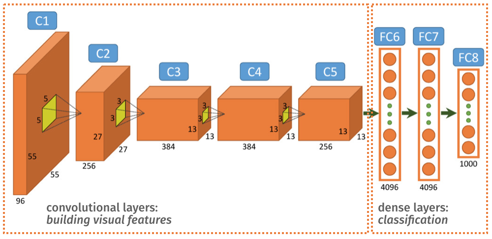
In broad terms, the convolutional layers (up to C5) are responsible for learning and extracting visual features from the input images. The final dense layers (FC6, FC7, and FC8) then use these features to perform classification.
Networks like AlexNet, VGG, ResNet, and GoogLeNet have been trained on vast datasets such as ImageNet, which contains millions of images across thousands of categories. As a result, the filters learned by their convolutional layers are highly generic and effective for a wide range of visual tasks. These features can be repurposed for your specific application.
Instead of training a new network to learn visual features, you can reuse the ones from a pre-trained model. The process involves taking a pre-trained network, removing its final classification layers, and replacing them with your own, specialised layers designed for your specific task.
Depending on the size of your training dataset, you might choose to redesign only the final layer (e.g., FC8) or several of the later layers (e.g., C5, FC6, FC7, FC8). Redesigning more layers requires a larger amount of training data.
If you have a sufficient number of training samples, you can also fine-tune the imported layers by allowing backpropagation to update their weights. This adapts the pre-trained features to better suit your specific application. If your dataset is small, it is generally better to freeze the weights of the imported layers to prevent overfitting.
In PyTorch, you can freeze the weights of a layer by instructing PyTorch not to update the weights during backprobagation. For instance, the following code freezes the all the weights in layer3 of model:
# Freeze weights in layer named `layer3`
for name, layer in model.named_children():
    if name in ['layer3']:
        for param in layer.parameters():
            param.requires_grad = False
For most image-based applications, it is highly recommended to start by reusing an off-the-shelf network. Research has shown that these generic visual features provide a strong baseline and can achieve state-of-the-art performance in many applications.
Razavian et al. ``CNN Features off-the-shelf: an Astounding Baseline for Recognition’’. 2014. https://arxiv.org/abs/1403.6382
7.1.2 Domain Adaptation and Vanishing Gradients
Reusing networks on new datasets can present challenges. Consider a single neuron with a \mathrm{tanh} activation function, f(x_i, w) = \mathrm{tanh}(x_i+w). Suppose the original network was trained on images taken on sunny days. The input values, x_i (red dots in Figure 7.2), are centred around 0, and the learned weight is \hat{w}=0.

Now, we want to fine-tune this network with new images taken on cloudy days. The input values for these new samples, x_i (green crosses), are now centred around 5. In this input range, the derivative of the \mathrm{tanh} function is close to zero, leading to the problem of vanishing gradients. This makes it extremely difficult to update the network weights effectively.
7.1.3 Normalisation Layers
To address this, it is crucial to ensure that the input data is within an appropriate value range. Normalisation Layers are used to scale the data according to the statistics of the training set, mitigating the effects of domain shift.
The output x_i' of a normalisation layer is given by:
x'_{i} = \frac{x_{i} - \mu_i}{\sigma_i}
where \mu_i and \sigma_i are the mean and standard deviation of the input data, computed offline.
After normalisation, the new samples are centred around 0, as shown in Figure 7.3, placing them in a region where the gradient of the activation function is large enough for effective learning.

7.1.4 Batch Normalisation
Batch Normalisation (BN) is a specific type of normalisation layer where the scaling parameters, \mu and \sigma, are determined as follows:
- During training, \mu_i and \sigma_i are the mean and standard deviation of the input x_i over the current mini-batch. This ensures that the output x_i' has a mean of 0 and a variance of 1.
- During evaluation, \mu_i and \sigma_i are the mean and standard deviation computed over the entire training set.
Batch Normalisation allows for higher learning rates and makes the network less sensitive to initialisation and other optimisation choices, such as Dropout.
Sergey Ioffe, Christian Szegedy. “Batch Normalization: Accelerating Deep Network Training by Reducing Internal Covariate Shift.” (2015) https://arxiv.org/abs/1502.03167
7.2 Going Deeper
The realisation that deeper networks could generalise better sparked a race to build increasingly deep architectures after 2012. The primary obstacle was the vanishing gradient problem, which made it difficult to train sequential architectures like VGG beyond 14-16 layers.
To better understand the key to mitaging this problem, consider the simple sequential network of Figure 7.4.

The gradient of the error with respect to a weight w is a product of intermediate derivatives:
\frac{\partial e}{\partial w} = \frac{\partial e}{\partial u_2} \frac{\partial u_2}{\partial u_1} \frac{\partial u_1}{\partial w}
If any of these intermediate derivatives is close to zero, the overall gradient \frac{\partial e}{\partial w} will also be close to zero, halting the learning process.
Now, let us replace the layer containing u_2 with a network of three units in parallel (u_2, u_3, u_4):

The gradient is now a sum of the gradients through these parallel paths:
\frac{\partial e}{\partial w} = \frac{\partial e}{\partial u_2} \frac{\partial u_2}{\partial u_1} \frac{\partial u_1}{\partial w} + \frac{\partial e}{\partial u_4} \frac{\partial u_4}{\partial u_1} \frac{\partial u_1}{\partial w} + \frac{\partial e}{\partial u_3} \frac{\partial u_3}{\partial u_1} \frac{\partial u_1}{\partial w}
With this architecture, it is much less likely that the overall gradient will vanish, as all three terms would need to be null simultaneously.
This principle of introducing parallel paths is a key innovation in modern deep learning and was central to the designs of GoogLeNet (2014) and ResNet (2015).
7.2.1 GoogLeNet: The Inception Module
GoogLeNet, the winner of the ILSVRC 2014 competition, achieved a top-5 error rate of 6.7%, which was close to human-level performance at the time. This 22-layer deep CNN introduced the Inception module, a sub-network that processes the input through multiple parallel convolutional pathways.
Szegedy et al. “Going Deeper with Convolutions”, CVPR 2015 (paper link)
Instead of a simple sequence of convolutional layers, GoogLeNet uses a series of Inception modules (as highlighted by the green boxe in Figure below).
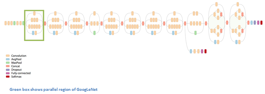
Each inception layer is a sub-network (hence the name inception) that produces 4 different types of convolutions filters, which are then concatenated (see this video for more explanations).
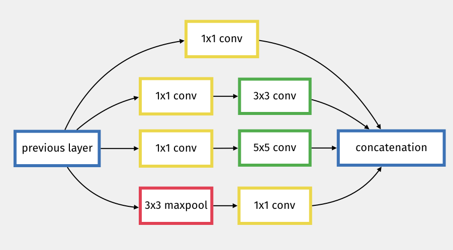
The Inception module creates parallel paths that mitigate the vanishing gradient problem, allowing us to go a bit deeper.
7.2.2 ResNet: Residual Connections
ResNet is a 152 (yes, 152!!) layer network architecture that won the ILSVRC 2015 competition with an error rate of just 3.6%, surpassing human performance.
Kaiming He et al (2015). “Deep Residual Learning for Image Recognition”. (paper link)
Similar to GoogLeNet, ResNet introduces parallel connections, but in a much simpler way. It uses residual connections, or skip connections, which add the input of a block of layers to its output.
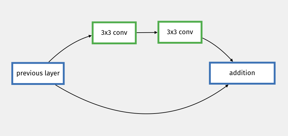
The idea is very simple but allows for a very deep and very efficient architecture. Skip connections can not only skip individual convolution blocks, but also entire parts of the network.
The ResNet architecture has been highly influential, and many pre-trained variants, such as ResNet-18, ResNet-34, and ResNet-50, are still widely used today.
7.3 A Modern Training Pipeline
7.3.1 Data Augmentation
It is often possible to artificially expand your dataset by generating variations of your existing input data. For images, common augmentation techniques include cropping, flipping, rotating, zooming, and adjusting contrast. These operations should not change the class of the image, so they provide a free and effective way to increase the size and diversity of the training set.
Similar techniques can be applied in other domains, such as adding noise, reverb, or compression to audio data.
Another approach is to synthesise data using simulation models, such as game engines. However, be aware that synthetic data is a simplified model of the real world and can lead to overfitting. It also tends to have different characteristics from real data, which can cause domain adaptation issues.
Generative models, such as those discussed in later chapters, can also be used to create synthetic data. For example, you could use a large language model to generate text for a natural language processing task.
7.3.2 Initialisation
Initialisation needs to be considered carefully. Starting with all weights at zero is generally a bad idea, as it can lead to being stuck in a local minimum with zero gradients from the outset. A better approach is to initialise the weights randomly. We need, however to be careful, and control the output at each layer to avoid a situation where gradients would explode or vanish through the different layers.
For networks using the ReLU activation function, He initialisation is a popular choice. For each layer l, the bias b and weights w are initialised as b_l=0, w_l\sim \mathcal{N}(0, \sqrt{2/n_{l-1}}), where n_{l-1} is the number of neurons in the previous layer. This helps to maintain a stable gradient flow throughout the network, at least at the beginning of training.
7.3.3 Optimisation
As discussed in previous chapters, various optimisation techniques are available for training. Adam and SGD with momentum are two of the most common choices. While Adam often converges faster, SGD with momentum has been shown to find local minima that generalise better. An improved version of Adam, called AdamW, has been proposed to address some of Adam’s shortcomings.
Another important aspect of optimisation is the learning rate schedule. Another aspect of the optimisation is the scheduling of the learning rate. It is generally beneficial to decrease the learning rate as the training progresses and the model approaches a local minimum.
In 2017 was popularised the idea of warm restarts, which periodically raise the learning rate to temporary diverge and allow to hop over hills. A variant of this scheme is the cosine annealing schedule shown in Figure 7.9.

An example of a reasonably modern optimiser setup in PyTorch might look like this:
import torch
import torch.nn as nn
import torch.optim as optim
from torch.optim.lr_scheduler import CosineAnnealingLR

# Assuming you have your model defined and initial_learning_rate and decay_steps
# For demonstration, let's assume some values
initial_learning_rate = 1e-3
decay_steps = 1000

# 1. Define your model
# model = MyModel(...)

# 2. Define the optimizer
optimizer = optim.AdamW(model.parameters(), lr=initial_learning_rate)

# 3. Define the learning rate scheduler
# T_max is the number of iterations for the first half of the cosine cycle.
scheduler = CosineAnnealingLR(optimizer, T_max=decay_steps, eta_min=0)

# 4. Training loop (simplified)
# for epoch in range(num_epochs):
#     for batch in dataloader:
#         optimizer.zero_grad()
#         # Forward pass, calculate loss
#         loss.backward()
#         optimizer.step()
#         scheduler.step() # Call scheduler.step() after optimizer.step()
7.3.4 Takeaways
Modern convolutional neural networks typically enhance the basic convolution-activation block with a combination of normalisation layers and residual connections. These additions make the networks more resilient to the vanishing gradient problem, enabling them to be much deeper and more effective for transfer learning.
A modern training pipeline usually includes data augmentation, an initialisation strategy (such as He or Xavier initialisation), a well-chosen optimiser (like AdamW), and a dynamic learning rate schedule (such as cosine annealing). Often, a transfer learning approach is used to kick-start the training process.
It is important to remember that there are no universal truths in deep learning. These are popular and proven techniques, but they may not be optimal for your particular application. Remember that experimentation and careful evaluation are part of your daily grind as a deep learning practitioner.