Alternative Matting Laplacian (Theory)

My paper on an alternative Matting Laplacian has been recently accepted at ICIP 2016. I have uploaded the preprint to arXiv.org and the reference code is also available on my github repository:

git clone https://github.com/frcs/alternative-matting-laplacian.git

Theory

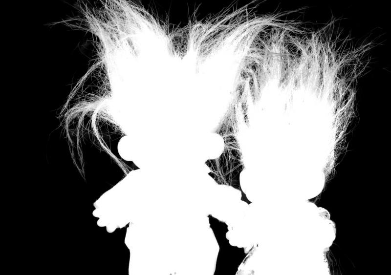
Consider the picture below (taken from www.alphamatting.com):

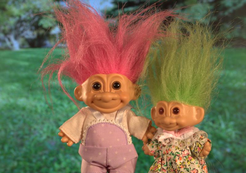
Say we want to cut out the trolls from the background. We need to extract an opacity mask of the foreground. This mask is called the $\alpha$ matte. When working in the linear RGB colour space, the observed colour $C_i$ at pixel $i$ is a blend between the foreground colour $F_i$ and the background $B_i$:

$C_i = \alpha_i F_i + (1 - \alpha_i) B_i$

We need to solve for $F_i$, $B_i$ and $\alpha_i$. This is unfortunately non-linear and over parameterised. In their remarkable work, Levin et al. propose that the transparency values can be approximated as a linear combination of the colour components:

$\alpha_i = a_i^T C_i + b_i$

with $a_i = [a_i^R, a_i^G, a_i^B]$. We can think of $a$ and $b$ as a colour filter that we apply on the picture to obtain an intensity map of $\alpha$. In a way, $a$ is the colour through which $\alpha$ is revealed. Below is as example with $\alpha=2.2 C^R -1.36 C^G - 0.41 C^B -0.04$:

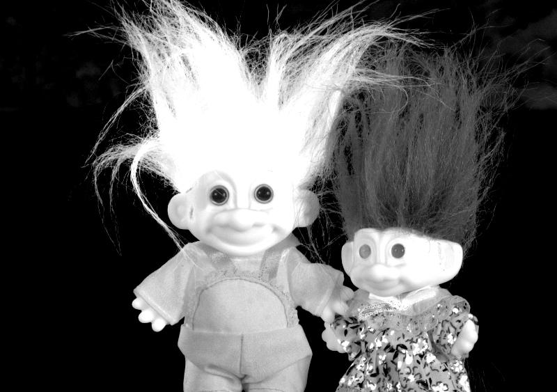
This map is a good approximation of $\alpha$ for the top left of the picture but not for the rest of the picture. Ideally then we would map a model to each pixel of the image. The problem is that we would end up with too many unknown parameters. Levin et al. solves this problem by introducing a spatial constraint that makes the problem tracktable and yields a global closed-form solution. They state that each local matting model should fit a local $3\times3$ image patch $w_i$ that overlaps with its neighbourhood:

$J(\alpha, a, b) = \sum_i \sum_{j\in w_i } \left(a_i^T C_j + b_i - \alpha_j\right)^2$

This is a quadratic expression in $a$, $b$ and $\alpha$. Levin et al. show that a closed-form solution for $\alpha$ can be found without having to explicitly compute the model parameters $a_i$ and $b_i$:

$J^*(\alpha) = \min_{a,b} J(\alpha, a, b)$

This leads to a sparse linear system $L \alpha = 0$, which can be solved using iterative solvers. It then is easy to add constraints to the values of $\alpha$. Below is a result based on this method:

Now, let us look at what the implicitly computed model parameters look like. The image below is a map of $a/5 + 0.5$:

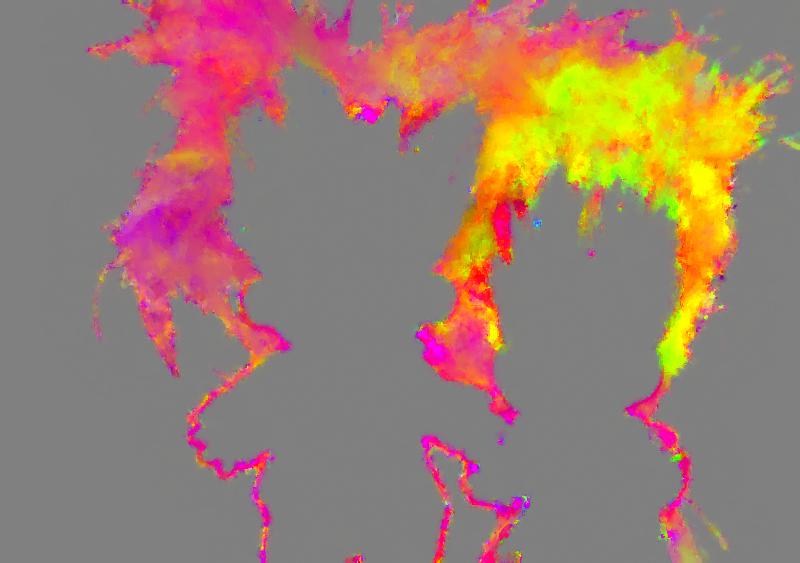
Recall that $a$ is in fact the colour through which we can reveal $\alpha$, thus what we see here are the colours (up to some brightness and contrast) of the local colour filter that is used to reveal $\alpha$ . What is striking is that $a$ shows some smoothness and we should try to exploit it. Unfortunately this is hard to do with Levin et al. as the model paremeters are not exposed in the equations.

Our contribution is to take the opposite approach of Levin et al. and explicitly solve for the model parameters instead:

$J^*(a,b) = \min_{\alpha} J(\alpha, a, b)$

We then show that a closed-form solution can also be found for $a$ and $b$. Interestingly the problem turns out to be an anisotropic diffusion of $a$ and $b$:

$\mathrm{div}\left( \left[ \begin{array}{c} C_i \\ 1 \end{array} \right] \left[ \begin{array}{cc} C^T_i & 1 \end{array} \right] \nabla \left[ \begin{array}{c} a_i \\ b_i \end{array} \right] \right) = 0$

This also leads to a sparse linear system $A [\begin{array}{cc} a & b \end{array}]^T = 0$. But since we have an explicit representation of the model parameters, it is now easier to add further smoothness priors to the model parameters. For instance below is the result of increasing the spatial smoothness of $a$:

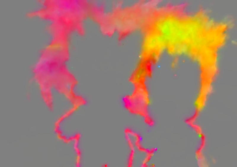
The resulting transparency map still shows little difference with Levin et al.:

The advantages of this approach are

1. Computational. Our equations are simpler than in Levin et al..
2. Modelling. It is easier to set meaningful priors on $a$ and $b$.